Introduction

The most common way to model complex smooth surfaces is by using a patchwork of bicubic patches such as BSplines or NURBS.

However, while they do provide a reliable smooth limit surface definition, bicubic patch surfaces are limited to 2-dimensional topologies, which only describes a very small fraction of real-world shapes. This fundamental parametric limitation requires authoring tools to implementat at least the following functionalities:

• smooth trimming
• seams stitching

Both trimming and stitching need to guarantee the smoothness of the model both spatially and temporally as the model is animated. Attempting to meet these requirements introduces a lot of expensive computations and complexity.

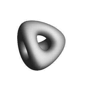
Subdivision surfaces on the other hand can represent arbitrary topologies, and therefore are not constrained by these difficulties.

Arbitrary Topology

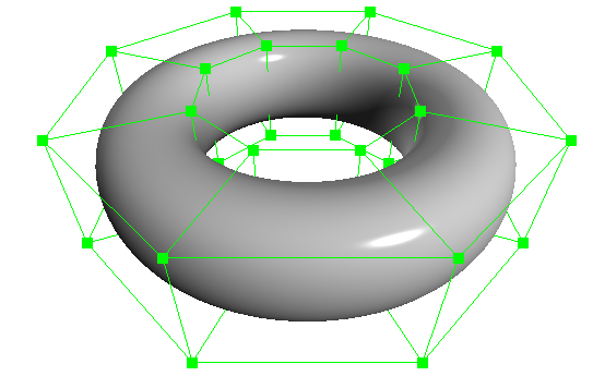
A subdivision surface, like a parametric surface, is described by its control mesh of points. The surface itself can approximate or interpolate this control mesh while being piecewise smooth. But where polygonal surfaces require large numbers of data points to approximate being smooth, a subdivision surface is smooth - meaning that polygonal artifacts are never present, no matter how the surface animates or how closely it is viewed.

Ordinary cubic B-spline surfaces are rectangular grids of tensor-product patches. Subdivision surfaces generalize these to control grids with arbitrary connectivity.

Manifold Geometry

Continuous limit surfaces require that the topology be a two-dimensional manifold. It is therefore possible to model non-manifold geometry that cannot be represented with a smooth C2 continuous limit. The following examples show typical cases of non-manifold topological configurations.

---

Non-Manifold Fan

This "fan" configuration shows an edge shared by 3 distinct faces.

With this configuration, it is unclear which face should contribute to the limit surface, as 3 of them share the same edge (which incidentally breaks half-edge cycles in said data-structures). Fan configurations are not limited to 3 incident faces: any configuration where an edge is shared by more than 2 faces incurs the same problem.

---

Non-Manifold Disconnected Vertex

A vertex is disconnected from any edge and face.

This case is fairly trivial: there is no possible way to exact a limit surface here, so the vertex simply has to be flagged as non-contributing, or discarded gracefully.

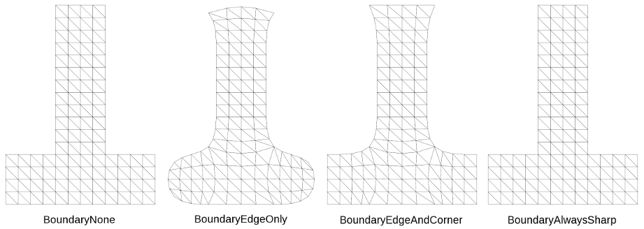
Boundary Interpolation Rules

Boundary interpolation rules control how boundary face edges and facevarying data are interpolated.

Vertex Data

The following rule sets can be applied to vertex data interpolation:

Mode	Behavior
0 - None	No boundary interpolation behavior should occur (debug mode - boundaries are undefined)
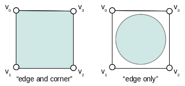
1 - EdgeAndCorner	All the boundary edge-chains are sharp creases and boundary vertices with exactly two incident edges are sharp corners
2 - EdgeOnly	All the boundary edge-chains are sharp creases; boundary vertices are not affected

On a quad example:

Facevarying Data

The following rule sets can be applied to facevarying data interpolation:

Mode	Behavior
0	Bilinear interpolation (no smoothing)
1	Smooth UV
2	Same as (1) but does not infer the presence of corners where two facevarying edges meet at a single faceA
3	Smooths facevarying values only near vertices that are not at a discontinuous boundary; all vertices on a discontinuous boundary are subdivided with a sharp rule (interpolated through). This mode is designed to be compatible with ZBrush and Maya's "smooth internal only" interpolation.

Unwrapped cube example:

Propagate Corners

Facevarying interpolation mode 2 (EdgeAndCorner) can further be modified by the application of the Propagate Corner flag.

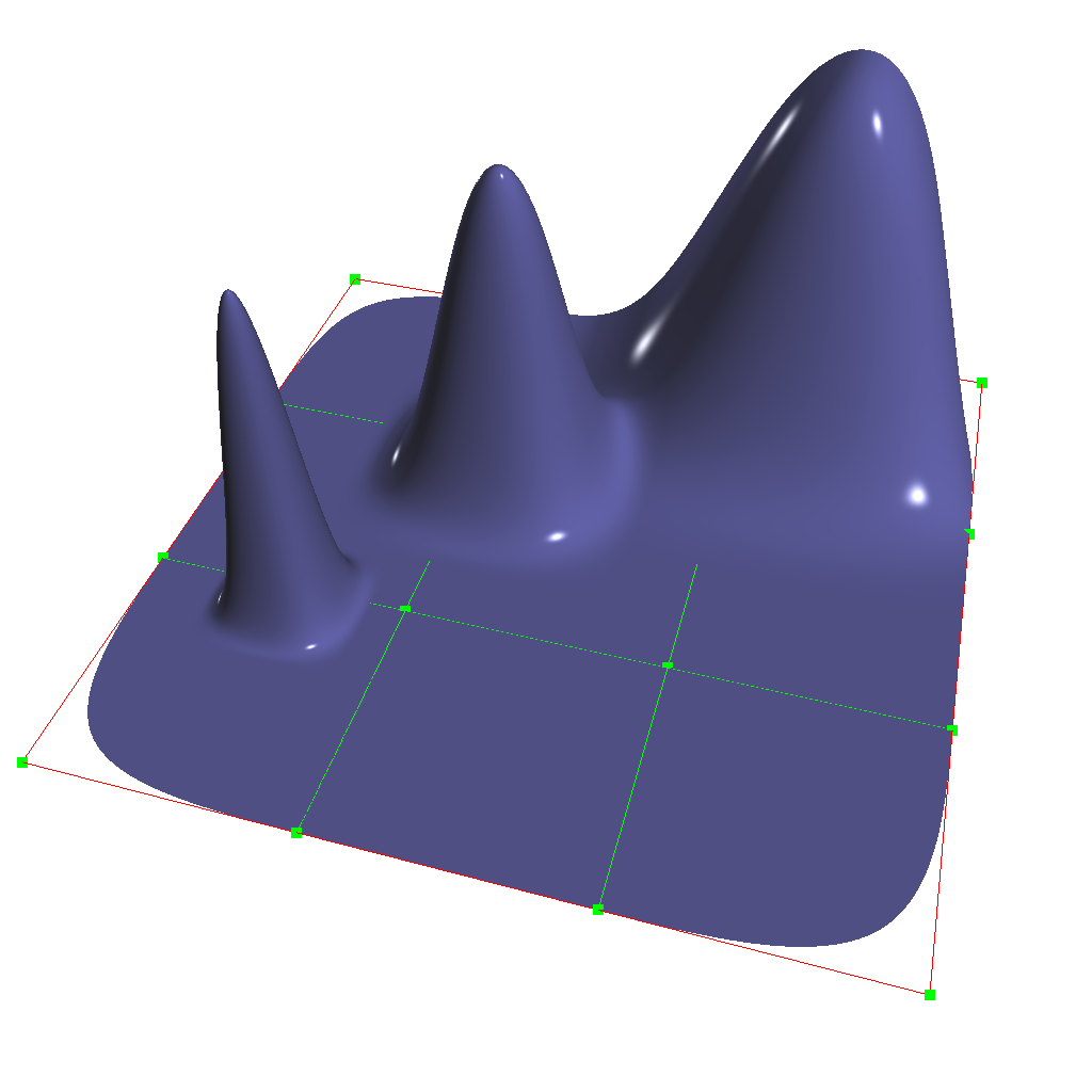
Semi-Sharp Creases

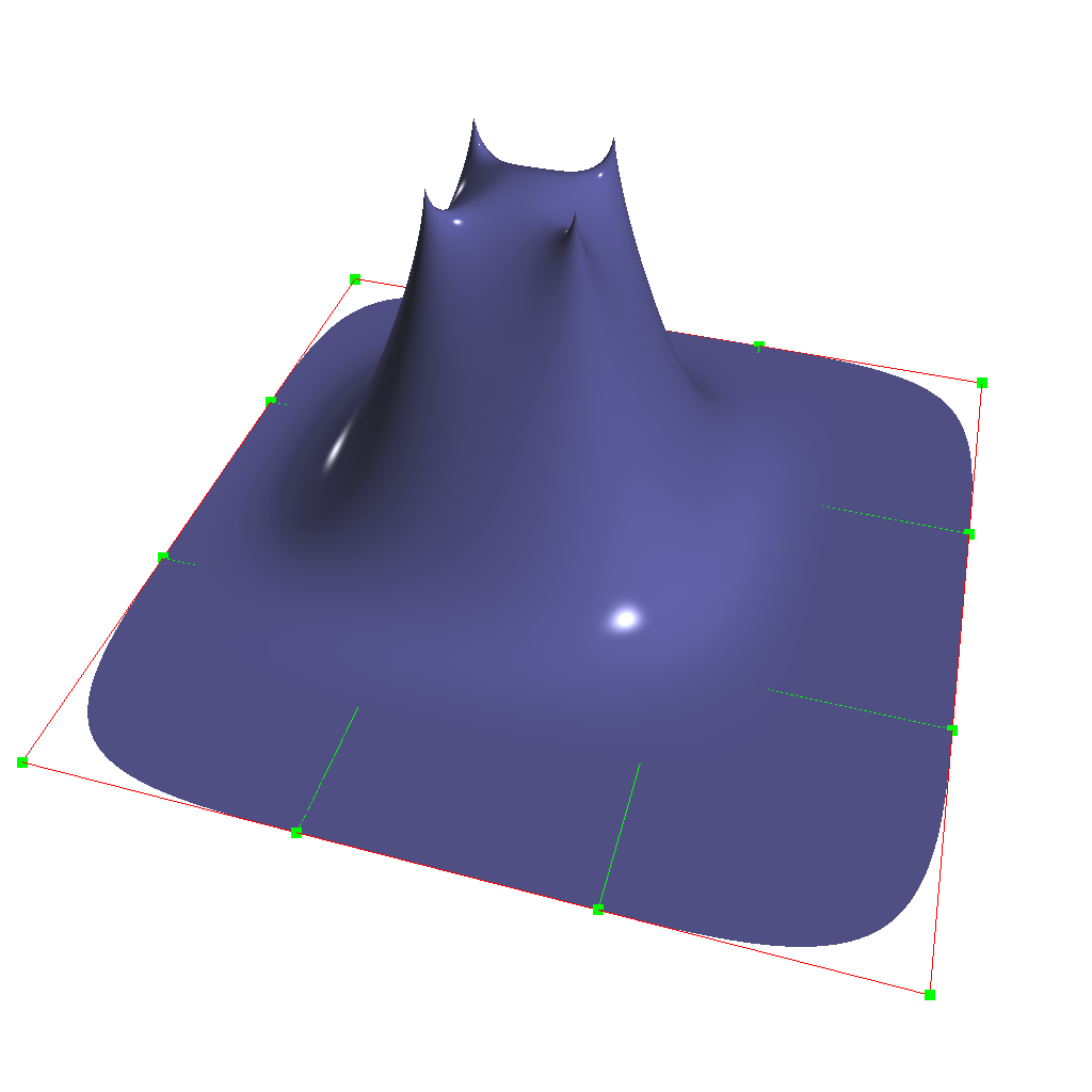
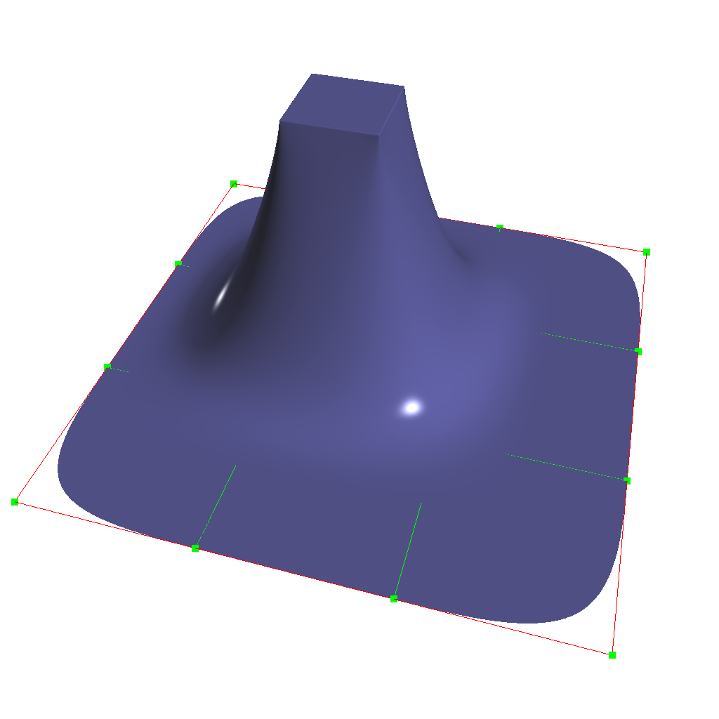
It is possible to modify the subdivision rules to create piecewise smooth surfaces containing infinitely sharp features such as creases and corners. As a special case, surfaces can be made to interpolate their boundaries by tagging their boundary edges as sharp.

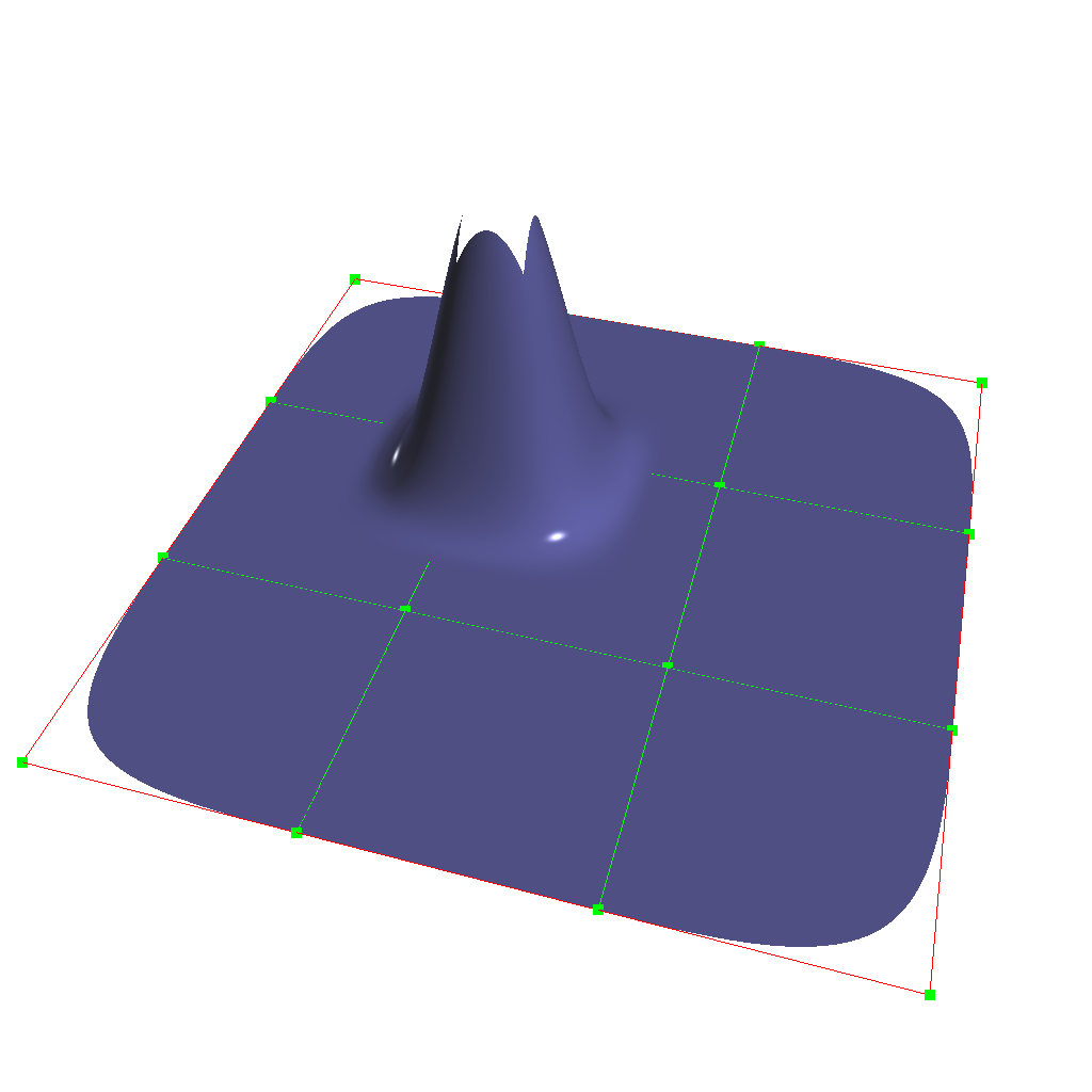
However, we've recognized that real world surfaces never really have infinitely sharp edges, especially when viewed sufficiently close. To this end, we've added the notion of semi-sharp creases, i.e. rounded creases of controllable sharpness. These allow you to create features that are more akin to fillets and blends. As you tag edges and edge chains as creases, you also supply a sharpness value that ranges from 0-10, with sharpness values >=10 treated as infinitely sharp.

It should be noted that infinitely sharp creases are really tangent discontinuities in the surface, implying that the geometric normals are also discontinuous there. Therefore, displacing along the normal will likely tear apart the surface along the crease. If you really want to displace a surface at a crease, it may be better to make the crease semi-sharp.

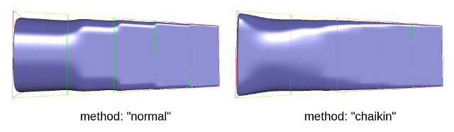
Chaikin Rule

Chaikin's curve subdivision algorithm improves the appearance of multi-edge semi-sharp creases with vayring weights. The Chaikin rule interpolates the sharpness of incident edges.

Hierarchical Edits

To understand the hierarchical aspect of subdivision, we realize that subdivision itself leads to a natural hierarchy: after the first level of subdivision, each face in a subdivision mesh subdivides to four quads (in the Catmull-Clark scheme), or four triangles (in the Loop scheme). This creates a parent and child relationship between the original face and the resulting four subdivided faces, which in turn leads to a hierarchy of subdivision as each child in turn subdivides. A hierarchical edit is an edit made to any one of the faces, edges, or vertices that arise anywhere during subdivision. Normally these subdivision components inherit values from their parents based on a set of subdivision rules that depend on the subdivision scheme.

A hierarchical edit overrides these values. This allows for a compact specification of localized detail on a subdivision surface, without having to express information about the rest of the subdivision surface at the same level of detail.

Hierarchical Edits Paths

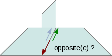
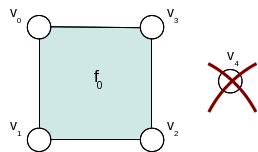
In order to perform a hierarchical edit, we need to be able to name the subdivision component we are interested in, no matter where it may occur in the subdivision hierarchy. This leads us to a hierarchical path specification for faces, since once we have a face we can navigate to an incident edge or vertex by association. We note that in a subdivision mesh, a face always has incident vertices, which are labelled (in relation to the face) with an integer index starting at zero and in consecutive order according to the usual winding rules for subdivision surfaces. Faces also have incident edges, and these are labelled according to the origin vertex of the edge.

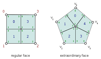
In this diagram, the indices of the vertices of the base face are marked in red; so on the left we have an extraordinary Catmull-Clark face with five vertices (labeled 0-4) and on the right we have a regular Catmull-Clark face with four vertices (labelled 0-3). The indices of the child faces are blue; note that in both the extraordinary and regular cases, the child faces are indexed the same way, i.e. the subface labeled n has one incident vertex that is the result of the subdivision of the parent vertex also labeled n in the parent face. Specifically, we note that the subface 1 in both the regular and extraordinary face is nearest to the vertex labelled 1 in the parent.

The indices of the vertices of the child faces are labeled green, and this is where the difference lies between the extraordinary and regular case; in the extraordinary case, vertex to vertex subdivision always results in a vertex labeled 0, while in the regular case, vertex to vertex subdivision assigns the same index to the child vertex. Again, specifically, we note that the parent vertex indexed 1 in the extraordinary case has a child vertex 0, while in the regular case the parent vertex indexed 1 actually has a child vertex that is indexed 1. Note that this indexing scheme was chosen to maintain the property that the vertex labeled 0 always has the lowest u/v parametric value on the face.

By appending a vertex index to a face index, we can create a vertex path specification. For example, (655 2 3 0) specifies the 1st. vertex of the 3 rd. child face of the 2 nd. child face of the of the 655 th. face of the subdivision mesh.

Vertex Edits

Vertex hierarchical edits can modify the value or the sharpness of primitive variables for vertices and sub-vertices anywhere in the subdivision hierarchy.

The edits are performed using either an "add" or a "set" operator. "set" indicates the primitive variable value or sharpness is to be set directly to the values specified. "add" adds a value to the normal result computed via standard subdivision rules. In other words, this operation allows value offsets to be applied to the mesh at any level of the hierarchy.

Edge Edits

Edge hierarchical edits can only modify the sharpness of primitive variables for edges and sub-edges anywhere in the subdivision hierarchy.

Face Edits

Face hierarchical edits can modify several properties of faces and sub-faces anywhere in the subdivision hierarchy.

Modifiable properties include:

• The "set" or "add" operators modify the value of primitive variables associated with faces.
• The "hole" operation introduces holes (missing faces) into the subdivision mesh at any level in the subdivision hierarchy. The faces will be deleted, and none of their children will appear (you cannot "unhole" a face if any ancestor is a "hole"). This operation takes no float or string arguments.

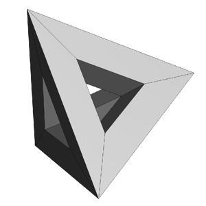
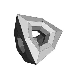
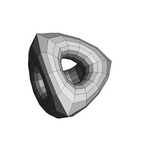
Uniform Subdivision

Applies a uniform refinement scheme to the coarse faces of a mesh. This is the most common solution employed to apply subdivision schemes to a control cage. The mesh converges closer to the limit surface with each iteration of the algorithm.

Feature Adaptive Subdivision

Generates bi-cubic patches on the limit surface and applies a progressive refinement scheme in order to isolate non-C2 continuous extraordinary features.

Uniform or Adaptive ?

Main features comparison: